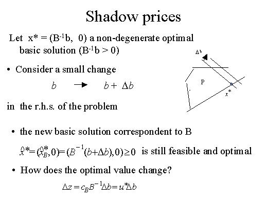
Denote by x* the optimal basic solution of the original instance of the
problem. x* corresponds to a particular submatrix B. Now consider a small
increment Db of one or more components
of the vector b.
If the changes are sufficiently small, the basic solution of the new problem
hatx* corresponding to the same matrix B is still feasible. In this case,
it is optimal for the new problem since a change in the r.h.s. does not
affect the reduced costs. Which is the value of the new optimal solution?
One easily derives that the new optimal value is equal to the old one
plus the quantity delataz given by the scalar product of Db
the dual optimal vector u*, which has not changed. From the last equality
we deduce the economic interpretation of the dual vector u*. Indeed this
equality says that each component of u* represents the increment in the
primal optimal value corresponding to an unit increase of the same component.
In other words, the optimal dual variables represent how much on looses
in the optimal value of the primal problem because of the rigidity of
each single constraint. For this reason the dual variables are also called
shadow prices or marginal prices.